There are various machine learning algorithms like KNN, Naive Bayes, Logistic Regression, Linear Regression, SVM, Ensemble models etc etc. But how do you measure the performance of these models ? Is there any one metric which will define how good a model is ? Well, in this blog I will discuss about the important KPIs (Key Performance Indicators) to measure the performance of a Machine Learning Model
- Accuracy
- Confusion matrix
- Precision, Recall & F1 score
- Receiver Operating Characteristic Curve (ROC)
- Log-loss
- R-Squared Coefficient
- Median absolute deviation (MAD)
- Error Distribution
Sample dataset: I will consider a sample test dataset to explain the metrices. The sample data contains 15 positive Y’s & 15 negative Y’s. It is a simple binary classification problem
P.S: We measure the performance of models based only on TEST data and NOT on train data/ cross-validation data.
Accuracy
Accuracy is the most easiest metric to understood & to implement as well. Accuracy is nothing but the ratio of correctly classified data points to the total number of data points.
Example: For the above sample dataset, if a model predicts 13 positive points & 14 negative points correctly, then
\[Accuracy = (13+14)/30\] \[Accuracy = 0.9\]Cons
-
Accuracy is a bad metric for a highly imbalanced dataset: Consider a highly imbalanced dataset like credit card fraud detection, where >99% of the data points are negative. Lets say we have very dumb model which will always predict negative, irrespective of given data points (i.e., X). And if we calculate the Accuracy for this dumb model, it would be more than 0.99 that means even a dumb model is showing an accuracy of 0.99 which is obviously wrong.
-
Can not take probability scores: Accuracy don’t take probability scores into consideration. It will just consider the predicted Y values. For example
Lets say we have two Models M1 & M2.
| ID | Y | M1_prob | M2_prob | M1_pred | M2_pred |
|---|---|---|---|---|---|
| 1 | 1 | 0.90 | 0.55 | 1 | 1 |
| 2 | 0 | 0.10 | 0.45 | 0 | 0 |
| 3 | 1 | 0.88 | 0.51 | 1 | 1 |
| 4 | 1 | 0.93 | 0.60 | 1 | 1 |
| 5 | 0 | 0.01 | 0.48 | 0 | 0 |
Where,
Y : real Y values
M1_prob: probability of Y = 1 for model M1
M2_prob: probability of Y = 1 for model M2
M1_pred: predicted Y values from model M1
M2_pred: predicted Y values from model M2
As we can see, both M1 & M2 models predicted the same Y’s & have same accuracy.But if you see probability scores of M1 & M2, the model M1 is performaning better than the model M2, since the probability scores are high for the M1 model, whereas for the model M2,the probability scores are almost half
Confusion matrix:
Confusion matrix is a matrix used to describe the performance of a classification model. It solves the problem the accuracy metric had with the imbalanced dataset
Lets consider a binary classification problem i.e., Y belongs to 0 or 1. 0 being negative label & 1 being positive label. Let Y be the actual values & Y^ be the predicted values
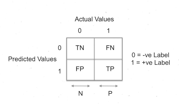
where,
TN (True Negative) : number of data points for which Y = 0 & Y^ = 0
FN (False Negative) : number of data points for which Y = 1 & Y^ = 0
FP (False Positive) : number of data points for which Y = 0 & Y^ = 1
TP (True Positive) : number of data points for which Y = 1 & Y^ = 1
Tip to remember: Here is a tip to remember which I learned from Applied AI course
Example: Lets consider the case Y = 0, Y^ = 0. Here predicted value is 0, i.e, Negative (N) & the it is correct (T) (since the actual value is also Negative). So it becomes True Negative (TN)
If we have a multi class classification, then confusion matrix size would be CxC, where C is the number of class labels.
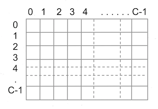
If the model you trained is very good, then all the principle diagonal values will be high & non-principle diagonal values will be low or zero.
Let P & N be the total number of Positive & Negative test data points respectively, Then
\[TPR (True Positive Rate) = TP/P\] \[TNR (True Negative Rate) = TN/N\] \[FPR (False Positive Rate) = FP/P\] \[FNR (False Negative Rate) = FN/N\]In layman language,
TPR = Percentage of correctly classified positive points
TNR = Percentage of correctly classified negative points
FPR = Percentage of incorrectly classified positive points
FNR = Percentage of incorrectly classified negative points.
Example: Consider a highly imbalanced dataset like credit card fraud detection, where >99% of the data points are negative. Lets say we have very dumb model which will always predict negative, irrespective of given data points (i.e., X). And if we calculate the Confusion matrix for this dumb model, then TNR will be 100 & TPR will be zero but FNR will be high which indicats the model is very dumb
In Confusion matrix we have 4 numbers, how one will know which one is important? Well, it depends on the dataset.
Example: If the dataset is cancer detection/credit card fraud detection, then we want high TPR and very less or 0 FNR.
Cons
- Can not take probability scores: Confusion matrix don’t take probability scores into consideration. It will just consider the predicted Y values.
Precision, Recall, F1 score
Precision & Recall are used in information retrieval, pattern recognition & binary classification. Please refer Wiki for info. Precision & Recall considers only the positive class labels.
\[Precision = \frac{TP}{FP+TP}\] \[Recall = \frac{TP}{FN+TP}\]In layman language,
Precision: Of all the predicted POSITIVE labels, how many of them are actually POSITIVE
Recall: Of all the actual POSITIVE labels, how many of them are correctly predicted as POSITIVE.
We always want Precision & Recall to be high. Precision & Recall values ranges from 0 to 1
F1 Score: It is a single measurement, which considers both Precision & Recall to compute the score. It is basically the harmonic mean of Precision & Recall. The value of F1 score ranges from 0 to 1.
\[F1 score = 2 *\frac{Precision*Recall}{Precision+Recall}\]This metric is extensively used in Kaggle compitations. But Precision & Recall is more interpretable or I can say F1 score is difficult to interpret.
Modification of F1 Score For Multi label classification
In Multi-label Classification, multiple labels may be assigned to each instance and there is no constraint on how many of the classes the instance can be assigned to. Source: Wiki
There are two variations of F1 Scores
Micro F1 Score:
Calculate metrics globally by counting the total true positives, false negatives and false positives.
Lets say we have C labels, then Micro F1 score is defined as
where,
\[{Precision_{micro}}=\frac{\sum_{k∈C}TP_k}{\sum_{k∈C}(TP_k + FP_k)}\] \[{Recall_{micro}}=\frac{\sum_{k∈C}TP_k}{\sum_{k∈C}(TP_k + FN_k)}\]This is a better metric when we have class imbalance since it does take into account about the label frequency
Macro f1 score:
It is the simple average of F1 scores of all labels. This does not take into account about the label frequency.
\[F1_{macro} = \frac{1}{|C|}\sum_{k∈C}F1Score_k\]For info on F1 score clickhere
Receiver Operating Characteristic Curve (ROC)
ROC curve is a curve which is created by plotting TPR agains FPR. ROC Curve metric is applicable only for binary classification. Here is step by step procedure to draw ROC curve.
Lets assume, the model which we are using gives some kind of scores like probability scores (pridict_prob) in such a way that increase in score indicates higher probability of data point belonging to class 1. Lets assume Y^ denotes the predicted probability scores
1 = POSITIVE class
0 = NEGATIVE class
STEP 1: Sort Y^ in descending order.
| X | Y (actual) | Y^ prob(Y==1) |
|---|---|---|
| \({x_1}\) | 1 | 0.94 |
| \({x_2}\) | 1 | 0.87 |
| \({x_3}\) | 1 | 0.83 |
| \({x_4}\) | 0 | 0.80 |
STEP 2: Thresholding (\(\tau\)).
For each of the probability scores (lets say \({\tau_i}\)) in Y^ columns, if Y^ >= \({\tau_i}\), then predicted label would be positive(1).
| X | Y (actual) | Y^ prob(Y==1) | Y_predicted \(\tau\) = 0.94 | Y_predicted \(\tau\) = 0.87 | Y_predicted \(\tau\) = 0.83 | Y_predicted \(\tau\) = 0.80 |
|---|---|---|---|---|---|---|
| \({x_1}\) | 1 | 0.94 | 1 | 1 | 1 | 1 |
| \({x_2}\) | 1 | 0.87 | 0 | 1 | 1 | 1 |
| \({x_3}\) | 1 | 0.83 | 0 | 0 | 1 | 1 |
| \({x_4}\) | 0 | 0.80 | 0 | 0 | 0 | 1 |
If we have N data points, then we will have N thresholds.
STEP 3: For each of the Y_predicted (\({\tau_i}\)), calculate TPR & FPR.
In our example
| X | TPR | FPR |
|---|---|---|
| \(\tau\) = 0.94 | 0.33 | 0 |
| \(\tau\) = 0.87 | 0.66 | 0 |
| \(\tau\) = 0.83 | 1 | 0 |
| \(\tau\) = 0.80 | 1 | 1 |
If we have N data points, then we will have N TPR,FPR pairs.
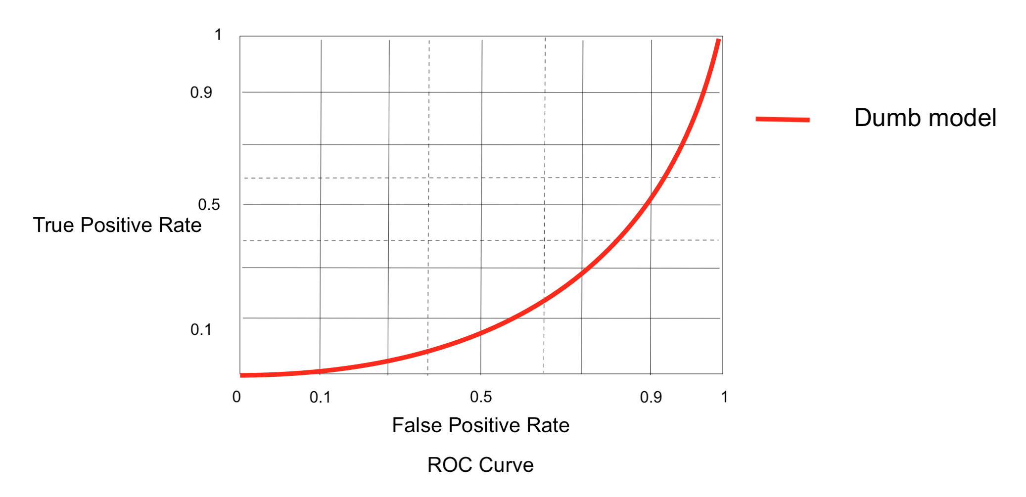
STEP 4: Plot TPR vs FPR by taking N TPR, FPR pair. Typically the Graph look like this
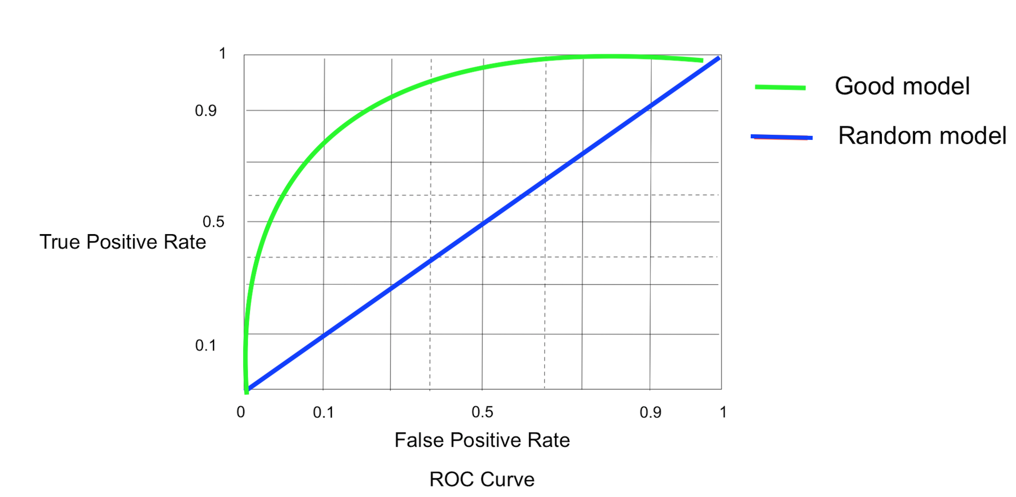
P.S: The example (TPR,FPR) pairs have not been plotted in the above graph
Random Model: Model which generates randomly 0 & 1’s
Good Model: Model which has high TPR & low FPR
Area Under ROC Curve (AUC): AUC is the area under the ROC curve. More the area under the curve, the more good is the model. A random model will have an AUC of 0.5
Cons
-
Imbalanced dataset: For an imbalanced dataset, a dumb model might give high AUC, which may be misleading sometimes.
-
Depends on the ORDERing of the scores & doesn’t depends the scores itself.
-
Works only for binary classification problems
Converting a dumb model into a reasonable good model
A dumb model is one which has AUC an < 0.5 In that case just swap class labels i.e., change 1 to 0 & 0 to 1 (Y_predicted = 1-Y_predicted) to make it a reasonably good model.
Log loss
It is an important metric & it uses probability scores to calculate the loss. This metric can be used for both binary classification & multi class classification. And it ranges from 0 to \(\infty\) (infinity). Log loss is a loss, so we always wants to minimize the losses. Lower the loss, the good is the model.
\[Log Loss = -\frac{1}{n}\sum_{i=1}^n \sum_{j=1}^c y_{ij}*log(p_i)\]where,
log = natural log
n = number of datapoints
c = number of class labels
\(y_{ij}\) = 1 if data point \(x_{i}\) belongs to class j else 0
\(p_{i}\) = probability of \(x_i\) belonging to class j
Example: Lets consider a binary classification dataset
| X | Y (actual) | Y^ prob(Y==1) |
log loss | log loss score |
|---|---|---|---|---|
| \({x_1}\) | 1 | 0.94 | -log(0.94) | 0.0269 |
| \({x_2}\) | 0 | 0.20 | -log(1-0.20) | 0.0969 |
| \({x_3}\) | 1 | 0.70 | -log(0.70) | 0.1549 |
| \({x_4}\) | 1 | 0.49 | -log(0.49) | 0.3979 |
As we can see from the above table, the data point \({x_1}\) is having higher probability of belonging to class label 1 & so its log loss is less comparitively, where as for the data point \({x_4}\), the log loss is higher because its probability is almost half, i.e., the probability of \({x_4}\) belonging to 1 or 0 is almost same.
Cons
Difficult to interpret the log loss score.
R-Squared Coefficient
This metric is used to measure the performance of a regression problem (Y belongs to real values). Lets Y^ denotes the predicted values & Y denotes the actual values.
| X | Y (actual) | Y^ |
|---|---|---|
| \({x_1}\) | 1.90 | 1.94 |
| \({x_2}\) | 1.34 | 1.20 |
| \({x_3}\) | 0.34 | 0.56 |
Sum of Squares (total): The simplest regression model one can build is the average model i.e, predicted value will be equal to average of all actual Y values.
\[{SS_{total}} = \sum_{i=1}^n (y- \overline{y})^2\]where, \(\overline{y}\) is the average of all y values
Sum of Squares (residual): Residual means the error, which is the difference between the predicted value & real value. Lets say y^ is the predicted value which is predicted using regression algorithms like linear regression.
\[{SS_{res}} = \sum_{i=1}^n (y-y\hat{}) ^2\]R Squared: It combines both \({SS_{total}}\) & \({SS_{res}}\)
\[R^2 = 1- \frac{SS_{res}}{SS_{total}}\]Case 1: \({SS_{res}} = 0\)
This is the best case ever could happen, i.e., predicted values are equal to actual values, so zero errors, therefore \(R^2 = 1\) for the best case
Case 2: \({SS_{res}} < {SS_{total}}\)
This means our model is performing better than the average model. The values of \(R^2\) ranges from 0 to 1.
Case 3: \({SS_{res}} = {SS_{total}}\)
This means our model is performing as good as the average model. So \(R^2 = 0\)
Case 4: \({SS_{res}} > {SS_{total}}\)
This means our model is performing worst than the average model. So \(R^2 < 0\)
Cons
\(R^2\) is not very robust to outliers
Median absolute deviation (MAD)
It overcomes the problem we had with \(R^2\). Median is robust to outliers
Median: It is the central tendancy or the midpoint of observed values
e: It is the difference between the actual value & the predicted value i.e,
\[e = y - y^\]MAD: It is the median of the absolute difference between the error (e) and the median of errors for all data points
\[MAD = median(|e - {median_e}|)\]where,
\({median_e}\) is the median of the errors
Error Distribution
By using PDFs & CDFs we can see the distribution of errors & so we can measure the performance of the models.
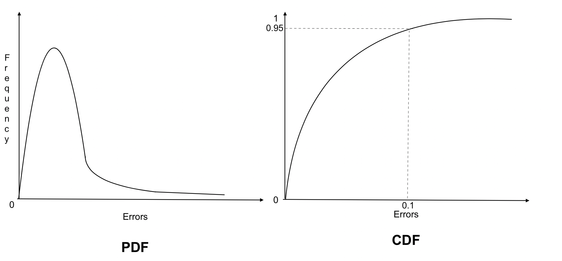
Observations:
PDF: As we can see, most of the errors are having smaller values where as few errors are having larger values
CDF: 95% of the errors are having the values less than 0.1 & only 5% of the errors are having values > 0.1.
Compare two models using CDFs of errors
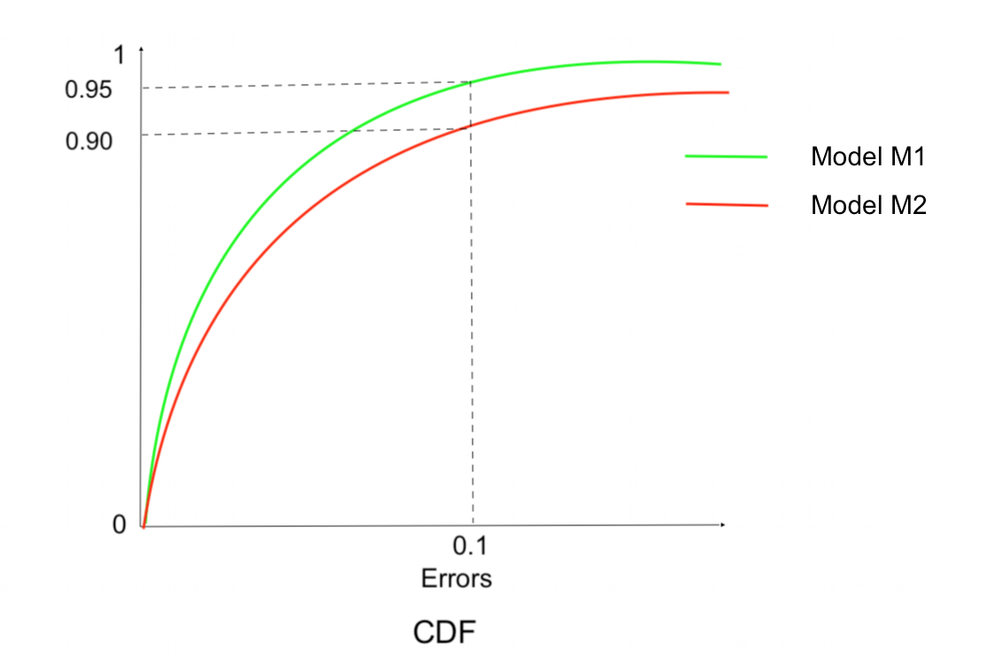
Model M1: 95% of the errors are having less than 0.1 value
Model M2: 90% of the errors are having less than 0.1 value
Since we always want errors to be zero or close to zero, Model M1 is better than Model M2, because more number of errors are close to zero in Model M1 than in Model M2
__
Thanks for reading. Please contact me regarding any queries or suggestions.