I had noticed for a long time that embedding models give high cosine similarity scores even for documents that have nothing in common. Two unrelated passages would come back at 0.74. I worked around it, moved on, and never dug into why.
Then I read this in the E5 model card FAQ:
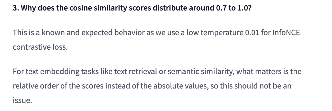
So it is known behaviour, and the reason given is a single training setting: a temperature of 0.01.
My working theory had always been that these models are overfitted on internet data. That was wrong. The model may well be overfitted on some data (yes, you still need to know underfitting, overfitting and the tradeoff in this AI era), but that is not why unrelated documents score high.
Digging into the real reason took me through anisotropy in transformer embeddings, the InfoNCE loss that almost every recent embedding model uses in some form, and what these models are actually optimised for. This post is everything I found.
The reason is that the loss function used to train these models only looks at the gap between scores, never at the scores themselves. It stops training once the gap is big enough, and at a temperature of 0.01 that works out to roughly 0.15. Everything above that gets left alone.
What you will learn
- What embedding models are actually optimised for, and why that matters
- What anisotropy is and how it puts a floor under every score
- How InfoNCE works, and why temperature decides your score range
- Why unrelated documents score 0.7 and above (the whole crux)
- How to fix it, and what to avoid
- How to set a threshold without guessing
Three teams say the same thing
E5 is not alone. The BGE model card says the same, in almost the same words:
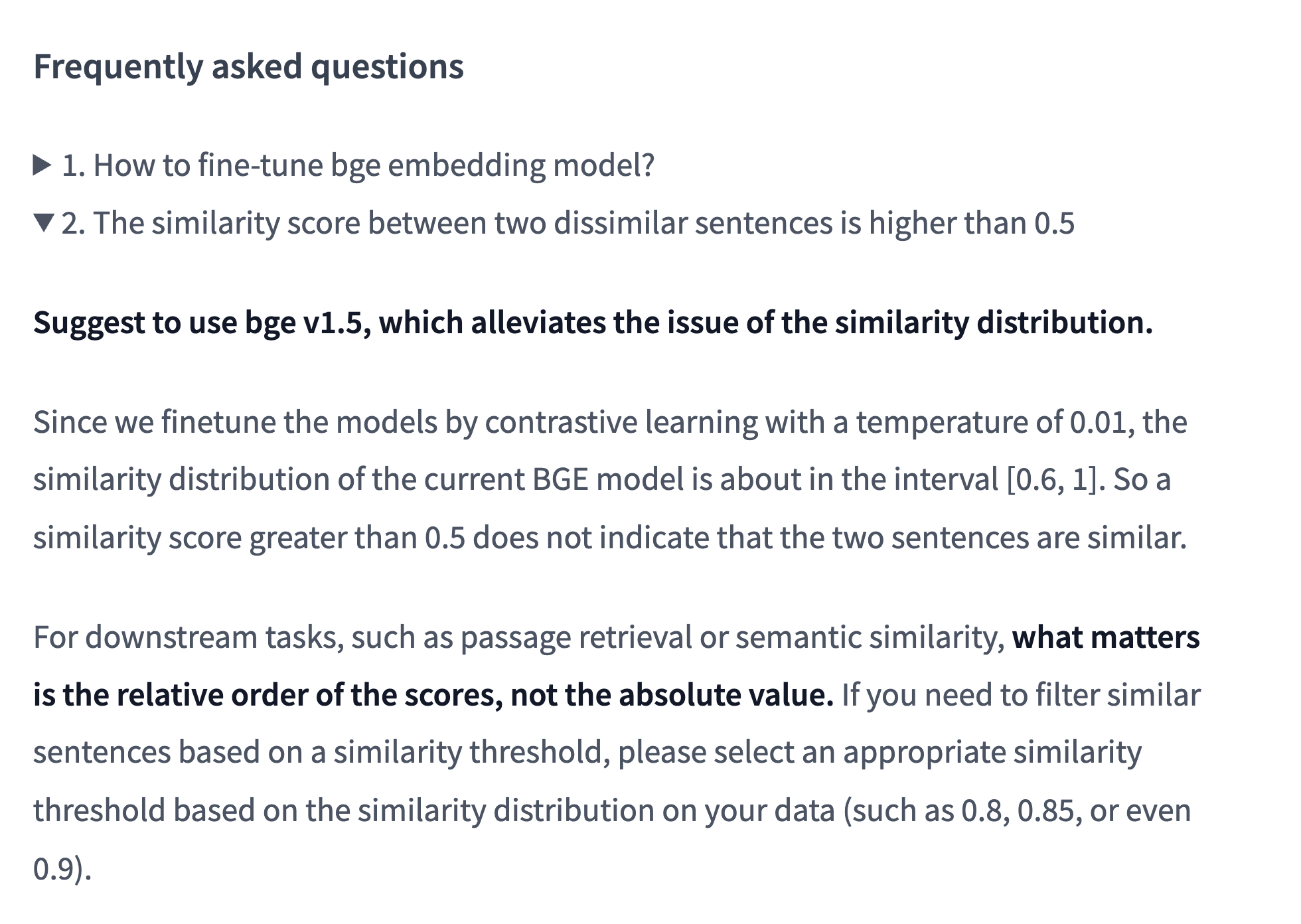
And when a user asked the GTE authors why any two of their embeddings score 0.75 or more, the answer was that the scores only capture which document is more relevant than which, and cannot be used as a measure of relevance.
Three separate teams, same temperature, same answer. The rest of this post is why that one setting does this.
How embedding models are trained
There is no single recipe, but most models built in the last couple of years follow roughly this shape.
1. Start from a pretrained model. Usually BERT or one of its variants. E5, for example, starts from bert-base-uncased.
2. Weak contrastive training (100M to 1B+ pairs). Train on pairs scraped from wherever pairs naturally occur, using InfoNCE with in-batch negatives only. No hard negatives. The point of this stage is cheap breadth, so the cleaning is minimal. Typical sources:
- Reddit (title and comment)
- StackExchange (question and accepted answer)
- Citation and abstract
- Wikipedia (section heading and definition)
- News (title and description)
- GitHub (code and docstring)
- Quora (question and answer)
- Amazon reviews (title and body)
- Datasets like MS MARCO, S2ORC, CommonCrawl
E5 collected 1.3 billion pairs this way and filtered them down to 270 million.
3. Supervised fine-tuning (1 to 2M pairs). Human labels, LLM generated and validated data, clean public datasets like SQuAD and Natural Questions, plus domain data. Aggressive cleaning and filtering. InfoNCE again, or InfoNCE combined with KL divergence to distil from a cross-encoder, with a much smaller batch size, for 1 to 3 epochs. This is the stage where good hard negatives get mined.
4. Whatever your end goal needs. Instruction support, Matryoshka embeddings, quantisation, and so on.
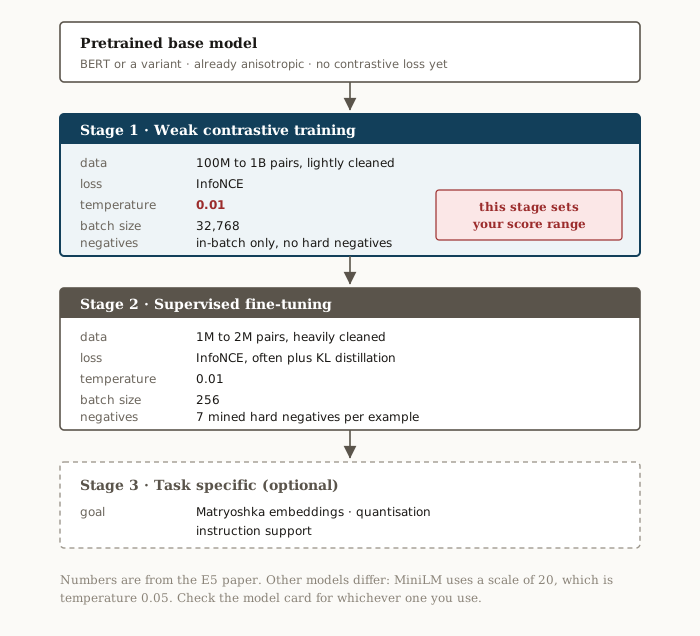
The numbers are from the E5 paper; stage 1 is where the score range is set.
Synthetic data from LLMs is what makes good hard negatives possible at scale, and hard negatives are what separate a decent embedding model from a good one.
Food for thought. If hard negatives are so useful, should we train on hard negatives only? No. A hard negative produces a large gradient, and a batch full of them pushes the optimiser in big jumps that overshoot. Tuning the learning rate helps, but mixing easy negatives in with the hard ones is the safer answer.
Anisotropy in transformer models
You would expect that when a transformer trains, every dimension of the embedding moves by roughly the same amount. That is not what happens. A small number of dimensions end up doing most of the work.
Timkey and van Schijndel (2021) found that often just 1 to 3 dimensions, out of the 768 a BERT-based model uses, carry far more spread than the rest, and those few end up deciding most of the cosine score. Ethayarajh (2019) measured the same thing from a different angle: the vectors do not spread out in all directions, they crowd into a narrow cone.
Both papers study word-level representations rather than sentence embeddings, so quote them for the base model rather than for BGE or E5 directly. But BGE, GTE, E5 and MiniLM all start from BERT or a BERT variant, so they inherit the cone before contrastive training even begins.
That still leaves a gap, because those papers measured individual words and you are comparing whole sentences. Pooling is what carries the problem across. A sentence embedding is built by combining the token vectors, usually by averaging them (E5) or by taking the first token (BGE). If a handful of dimensions hold large values in most token vectors, averaging keeps them large, and the sentence vector inherits the same lean.
Think of a cup of pencils. They fan out, no two point the same way, but every single one leans upward because they are sitting in the same cup. Pick two at random and the angle between them is small. Not because the pencils are related. Because they are all leaning.
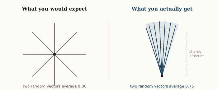
Cosine similarity compares two embeddings dimension by dimension and adds it all up. If a few dimensions hold large values in every embedding, those dimensions contribute a large positive amount to every single comparison, no matter what the two texts say. The model is not claiming the two sentences mean the same thing. The score is just dominated by the part where all texts look alike.
How far off is this? Take two genuinely random directions in 768 dimensions. The cosine between them averages 0, and it moves by only about 0.036 either side. So a neutral model would put unrelated text at 0.00, give or take 0.04. Real models put it at 0.75, which is about twenty times further out than random chance ever gets you.
So the starting point explains why unrelated text already scores high. But contrastive training runs for months on hundreds of millions of pairs, and the whole point of contrastive training is to separate things that should not look alike. Why does none of that fix it?
What embedding models are actually optimised for
One line I read while researching this stuck with me, and it is the real answer:
Embedding models are not optimised to push negatives as far away as possible from positives. They are optimised to rank good pairs above bad pairs. It is like a running race. The goal is to finish ahead of the others, not to maximise the time gap between first and second place.
Embedding models are optimised for ranking, not for scoring. The score is a byproduct.
And the model stops learning, more or less, the moment the objective is met. If a good pair scores 0.90 and a bad pair scores 0.75, the objective is already reached. Nothing in the loss then asks the model to drag that 0.75 down to zero, because that was never the goal.
You can see this in the naming. The sentence-transformers library calls its main contrastive loss MultipleNegativesRankingLoss. Not MultipleNegativesScoreLoss.
And the documentation says exactly what the objective is:
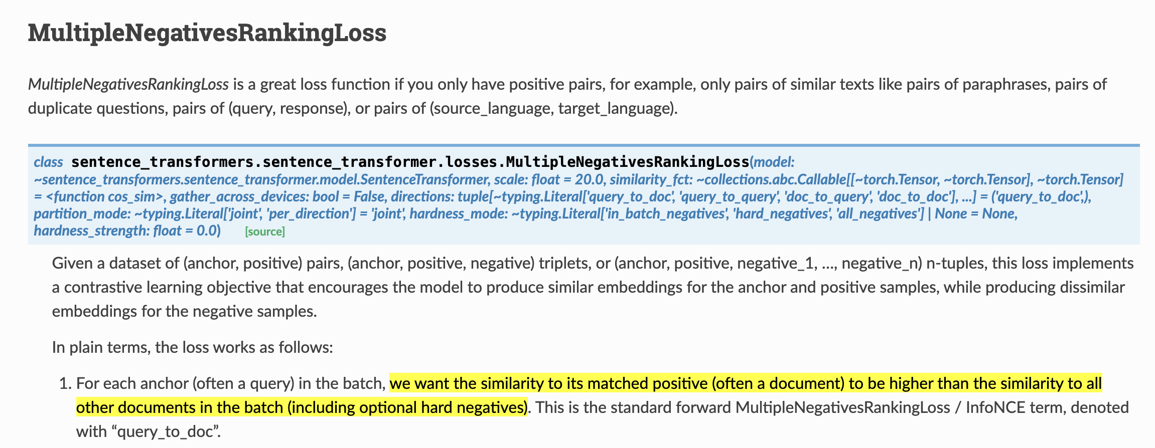
The wording is higher than. There is no mention of how much higher, or of what value either score should take.
This is also why triplet loss behaves differently. Triplet loss uses one negative at a time and an explicit margin you choose. InfoNCE uses every other item in the batch as a negative and gets its effective margin from the temperature instead. Both are ranking losses. Neither has a term that says “put negatives near zero”.
InfoNCE and contrastive learning
Once the base model is chosen, the next step is to apply InfoNCE (Information Noise Contrastive Estimation, from van den Oord et al. 2018) over 100M to 1B pairs. The same loss reappears at later stages with cleaner data.
InfoNCE frames contrastive learning as a classification problem. Given an anchor, pick which of N candidates is the positive. The other N-1 are negatives.
\[\mathcal{L}_{\text{InfoNCE}}=-\log\frac{\exp(\operatorname{sim}(\mathbf{q},\mathbf{k}^{+}))/\tau}{\sum_{i=1}^{N}\exp(\operatorname{sim}(\mathbf{q},\mathbf{k}_i)/\tau)}\]where:
- q is the anchor representation
- $\mathbf{k}^{+}$ is the positive representation
- $\mathbf{k}_{i}$ are the $N$ candidate representations, including the positive
- sim is a similarity function, usually cosine
- τ is the temperature
Written with the positive pulled out of the sum:
\[\mathcal{L}=-\log\left[\frac{\exp(s_{+}/\tau)}{\exp(s_{+}/\tau)+\sum_{j}\exp(s_{j}/\tau)}\right]\]where $s_{+}$ is the cosine with the correct passage and $s_{j}$ is the cosine with wrong passage j.
Divide the top and bottom by exp(s₊/τ)
\[\mathcal{L}=\log\left[1+\sum_{j}\exp\left(-\frac{s_{+}-s_{j}}{\tau}\right)\right]\]Every absolute score cancels out here. What is left depends only on the differences $s_{+} - s_{j}$.
The loss cannot see where your scores sit. Positives at 0.90 with negatives at 0.75 gives the same loss as positives at 0.30 with negatives at 0.15. Both have a gap of 0.15. The loss has no way to tell them apart, so it has no reason to prefer one over the other.
Let Δ be the gap
Assume every negative sits the same distance below the positive, so $\Delta = s_{+} - s_{j}$ for all j. Then the sum becomes N copies of one term:
\[\mathcal{L}(\Delta) = \log\left(1 + N e^{-\Delta/\tau}\right)\]And since $\mathcal{L} = -\log(p_{+})$, which runs from $0$ (when $p_{+} = 1$) to $\infty$ (when $p_{+} = 0$):
\[p_{+} = \frac{1}{1 + N e^{-\Delta/\tau}}\]Solving for Δ
Let ε be the loss we are aiming for, and let $X = N e^{-\Delta/\tau}$.
\[\log(1 + X) = \varepsilon\]For a small loss we can use the standard approximation log(1 + X) ≈ X. (Sanity check: if X = 0.01, then log(1.01) = 0.00995. Close enough.)
So X ≈ ε, and we can solve for Δ:
\[\begin{aligned} N e^{-\Delta/\tau} &= \varepsilon \\[2pt] e^{-\Delta/\tau} &= \varepsilon / N \\[2pt] -\Delta/\tau &= \ln(\varepsilon / N) \\[2pt] \Delta/\tau &= \ln(N / \varepsilon) \\[2pt] \Delta &= \tau \ln(N / \varepsilon) \end{aligned}\]Now put the real numbers in
E5 pretrains with τ = 0.01 and a batch size of 32,768, which means about 32,767 wrong answers per step. Aim for a loss of 0.01:
\[\Delta = 0.01 \times \ln(32768 / 0.01) = 0.01 \times 15.0 = \mathbf{0.150}\]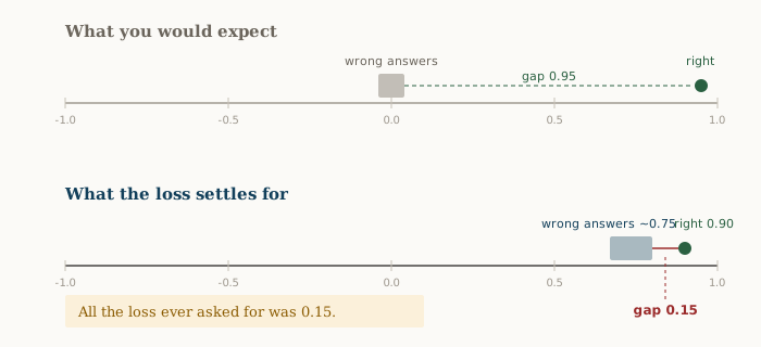
So the model has to get the right answer 0.15 ahead of 32,000 wrong ones. On a scale that runs from -1 to 1, that is not much to ask.
It starts with everything sitting around 0.75, inherited from BERT. So it lifts the right answer to 0.90 and the job is done. The loss is satisfied. There was never any reason to drag the wrong answers down to zero.
That 32,768 is generous, though. Because of the exp in the loss, the sum is dominated by a few near misses, so the real number is closer to a handful. The thousands of random passages get almost no push at all.
That 0.75 is not something the model did. It is something the model was never asked to undo.
Play with it
Move the sliders and watch where training stops caring.
What each setting does
Temperature decides how far apart the two groups end up. At 0.01 the loss accepts a gap of 0.15, so the model leaves both groups close together and both high, and you get scores packed into 0.7 to 1.0. At 0.05 the loss asks for a gap of 0.75, so the model has to force the groups apart and the scores spread out. Double the temperature and the gap it asks for doubles exactly. This is the setting that controls your score range.
Batch size changes the score range very little. N sits inside a logarithm. Going from 8 wrong answers to 262,144 moves the required gap from 0.067 to 0.171. You made the batch 32,000 times bigger and got 2.5 times more gap.
So why use 32,768? Not for the scores. For the wrong answers themselves. Among 8 random passages, none is close enough to confuse the model, so it already ranks them right and learns nothing. Among 32,768, a few dozen will be genuinely hard. A big batch hands you hard examples for free, without searching the whole corpus to find them. There is a second reason too: with only 8 wrong answers, one wrongly labelled document can take almost the entire training step. With 32,768 it cannot.
The gap cannot go past about 1.0. The best case is the right answer at 1.0 and the wrong answers at 0.0. You cannot do better, because the wrong answers are also each other’s wrong answers, so they have to spread out among themselves and cannot all sit below zero. This puts a ceiling on temperature. Above roughly 0.067 at N = 32,768, the loss asks for a bigger gap than cosine can give and is never satisfied.
The loss drops to zero quickly, not slowly. Once the gap it asked for is reached, the loss falls away fast, and no loss means no gradient. At τ = 0.01 this happens at 0.15, so the model stops there and everything beyond is left alone.
Why not just raise the temperature?
The field has had this option all along and has consistently not taken it.
The push each wrong answer receives is proportional to exp(δ/τ), where δ is how much closer it is than another wrong answer. Two negatives 0.05 apart get pushed in a ratio of 1.3 to 1 at τ = 0.2, but 148 to 1 at τ = 0.01. So a low temperature sends almost the entire training signal to the handful of wrong answers that nearly won. Those near misses are exactly what decides your ranking metrics. Wang and Liu (2021) study this tradeoff in detail.
E5, BGE and GTE were built by separate teams competing on the same public benchmarks. All three chose 0.01, and all three document the compressed score range in their own model cards. Three groups independently passing up an obvious readability win tells you something, even though none of them published the ablation.
MiniLM and most sentence-transformers models use a scale of 20, which is the same as τ = 0.05. So their scores do spread wider. Different models sit at different points on this tradeoff, which is one more reason not to reuse a threshold across models.
Measure it on your own data
Everything above explains why unrelated text scores high. None of it tells you where your scores sit, and that changes with every model and every corpus. A pile of cardiology papers all share medical language, so their unrelated pairs score higher than a mixed corpus. The E5 card says 0.7 to 1.0 and the BGE card says 0.6 to 1.0, but neither was measured on your data.
Sample a few thousand documents and score random pairs. Two documents picked at random are almost certainly unrelated, so these scores are your unrelated-pair distribution:
E = normalize(embed(["passage: " + t for t in sample]))   # ~5000 docs
i, j = random_pairs(len(E), 200_000)
unrelated = (E[i] * E[j]).sum(1)

print(unrelated.mean())   # e.g. 0.74
print(unrelated.std())    # e.g. 0.05
The mean is an average, not a minimum. Half your unrelated pairs score above it, so it is not a threshold. The standard deviation is what tells you where to put one. At 0.74 with a spread of 0.05, a few unrelated pairs will reach 0.89 by chance alone, and your cutoff has to clear those, not the average.
A shortcut for the first number: average all your embeddings into one vector and square its length.
mu = E.mean(0)
print(mu @ mu)        # 0.74, in one pass
This is exact rather than sampled, because averaging is linear. It saves you nothing when setting a threshold, but it does prove where the high scores come from. That one shared vector accounts for the whole 0.74. The model is not saying those documents are similar. You are measuring the part every document has in common.
Then track how far your real matches sit above the unrelated ones, counted in standard deviations:
z = (average of true pairs - average of unrelated pairs) / standard deviation of unrelated pairs
Track z rather than the raw score, because it survives rescaling. If some change halves both your unrelated average and your standard deviation, z does not move, and neither has the model improved. Only the numbers on the dial changed.
Solutions
1. Use the model as a ranker. If your application allows it, use the order and ignore the number. That is what the model was optimised for, and it costs you nothing.
2. Add a cross-encoder reranker. If latency allows. A cross-encoder reads the query and document together and is trained on relevance labels, so its scores mean something. It only reorders what you give it, so retrieve generously first.
3. Use the gap, not the value. Compare the score at position k with the score at k-1. A clear drop means you have run out of good results. If the scores are close, keep going down. What counts as a clear drop is something you measure on your own data.
4. Set any threshold from your own distribution. You already measured it above. Decide how many wrong results per query you can live with, then read the cutoff off that distribution rather than off a number you remember. And never carry a threshold across models or corpora. MiniLM, BGE, GTE and E5 all give high scores for unrelated text, but the ranges differ, and every corpus shifts them again. A cutoff of 0.8 is meaningless without knowing where your unrelated pairs sit.
5. Subtract the mean embedding. Take a sample from your full dataset, embed it, take the mean column wise, and subtract that mean embedding from every embedding. This removes the information that all your documents have in common, which is the shared direction described earlier.
One step people miss: after subtracting the mean, scale each vector back to length 1. Vector databases like Qdrant, Milvus and Pinecone use dot product for search and assume your vectors are already length 1. Skip the rescale and dot product stops matching cosine, so your results quietly get worse with no error to tell you.
Whether it helps at all depends a lot on whether the model was trained on data like yours. If it was, the shared direction may be carrying real signal and removing it can hurt. If it was not, you are mostly removing noise. There is no way to know in advance, so test it against your own retrieval metric before shipping it.
6. Train a small model instead. If your task is classification rather than search, SetFit needs only 8 to 16 examples per class and trains in minutes on CPU. A classifier outputs calibrated probabilities by construction, which removes the threshold problem rather than working around it.
7. Combine retrievers by rank, not by score. If you mix dense retrieval with BM25 using something like 0.5 * dense + 0.5 * bm25, dense scores move across a range of about 0.3 while BM25 moves across tens. BM25 decides everything and you will not notice. Use the position in each list instead of the raw number.
One thing to avoid in all of this: do not report the score to a user as a confidence percentage. It is not a probability and was never trained to be one.
Conclusion
The high scores are not a bug and not overfitting. There are two causes.
The base model starts with all its vectors leaning in one shared direction, so every pair of texts already scores high before training starts. Then contrastive training, which could have fixed that, never asks it to. The InfoNCE loss only looks at the gap between scores, and at τ = 0.01 with a large batch it is satisfied by a gap of about 0.15. The model reaches that gap by lifting the positive, the loss goes quiet, and the rest of the scores stay where they were.
So you can rely on the ordering these models give you. You cannot rely on the numbers. They are a byproduct of a ranking objective, and no part of the training ever fixed what they should be.
Which means the fix is not to hunt for a better threshold. It is to stop depending on the absolute number: use the order, rerank when accuracy matters, and set any cutoff from your own measured distribution.
And measure your own corpus before you do any of it. It takes 15 minutes and it will tell you more than any blog post, including this one.
References
- van den Oord, Li and Vinyals, Representation Learning with Contrastive Predictive Coding (2018). Where InfoNCE comes from.
- Ethayarajh, How Contextual are Contextualized Word Representations? (2019). Where the cone was first measured.
- Wang and Isola, Understanding Contrastive Representation Learning through Alignment and Uniformity on the Hypersphere (2020).
- Wang and Liu, Understanding the Behaviour of Contrastive Loss (2021). Temperature and hard negatives.
- Timkey and van Schijndel, All Bark and No Bite: Rogue Dimensions in Transformer Language Models (2021).
- Wang et al., Text Embeddings by Weakly-Supervised Contrastive Pre-training (2022). The E5 paper.
- Xiao et al., C-Pack: Packed Resources For General Chinese Embeddings (2023). The BGE paper.
- Sentence Transformers: MultipleNegativesRankingLoss
- Model cards: E5, BGE, and the GTE discussion thread