Key takeaways from building multiple machine learning models

Here is a list of my major key takeaways from doing various machine learning & deep learning experiments and reading several research papers and going through the courses. etc.

Weight initialization

1. weight initialization from uniform distribution or normal distribution N(0, σ). Pick σ depending on fan-in and fan-out (xavier glorot initialization, He initialization)

2. For the sigmoid activation function, xavier glorot initialization works well

3. For the ReLU activation function, He normal initialization works well.

Normalisation / Batch-normalisation

1. Data normalization is mandatory for DL problems.

2. Batch normalization helps in faster convergence & avoids internal covariance shit and we can try deep-layer networks.

3. “Batch-normalisation” at the later/last few layers works well.

SGD/Momentum

1. Functions having single minima or maxima are called convex functions (Ex: y=x²)& functions with multiple minima or maxima are called non-convex functions(Ex: y=x³)

2. Traditional algorithms work well for convex functions & deep learning works well for both.

3. Batch-wise SGD is an approximation to the standard GD

4. SGD is very slow & we have “sgd with momentum” (exponential weightage to previous grads), “Nestor accelerate moment” to make it faster.

Learning Rate algorithms

1. idea: decrease the learning rate as the iteration increases since we will be moving closer to the solution & we don’t want to bipass it and take U turn

2. learning rate varies for each feature depending on gradients calculated: AdaGrad (adaptive gradients), ada delta, adam (Adaptive moment estimation). In stats, 1. mean is called the first-order moment 2. variance is called the second-order moment

Activation Function

1. Sigmoid function: values of the sigmoid function ranges from 0 to 1 & its derivate ranges from 0 to 0.25. Using sigmoid , might lead to a vanishing gradient problem

2. Tanh function:values of the sigmoid function ranges from -1 to 1 & its derivate ranges from 0 to 1. Using tanh , might lead to a vanishing gradient problem. And if the weights are large, it might lead to exploding gradient

3. ReLU function: values of the sigmoid function ranges from 0 to +∞ & its derivate value would either be 0 or 1. 1. There won’t be any problems of vanishing gradient or exploding gradient. 2. There might be dead neuron problem since it all boils down to should we subtract learning rate from the old weight! 3. We can use leaky relu to solve the dead neuron problem

4. GeLU function:There are used in BERT, GPT-2 and most of the transformer based models.GeLU is a smoother version of ReLU and GeLU has a probabilistic interpretation.

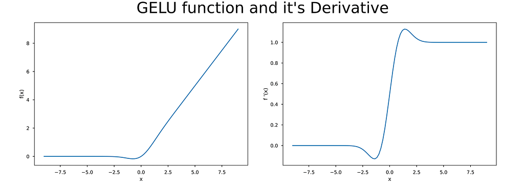
credit: https://alaaalatif.github.io/2019-04-11-gelu/

Metrics

1. AUC, accuracymetrics can be misleading on imbalanced datasets

2. the weighted macro-average f1 score is another way of computing the micro-average f1 score

3. micro-average f1 score can be a useful measure when the dataset varies in size.

Miscellaneous

1. parameters vs hyper-parameters: parameters are learned using the objective function & hyper-parameters are not part of objective functions (ex: learning rate)

2. If the loss at epoch e greater than the previous epoch’s loss e-1 , then ignore the updates made during the epoch e and load the weights from e-1 & reduce the learning rate (maybe by half) & start the next epoch. (brilliant explanation here)

3. Auto-encoders are really good at dimensionality reduction. It requires no supervised training data.

4. The validation set will be useful for hyper-parameter tuning & choosing NN architecture. But before exposing the model to real-world data, it should be retrained using all the available training datasets.

5. The Embedding layer` is as same as the Denselayer functionality-wise but the Embedding layer is a bit faster (refer to this link)

6. In eager execution, operations are evaluated immediately. In graph execution, a computational graph is constructed for later evaluation. Tensorflow defaults to eager execution

Visualizing Your Embeddings (SNE, t-SNE, UMAP)

1. SNE & t-SNE use KL divergence as the loss function

2. SNE & t-SNE use gradient descent with random initialization in the low dimensions

3. KL divergence loss doesn’t penalize for placing points, which are further away in high dimensions, closer to each other in low dimensions (major disadvantage)

4. SNE tries to keep similar points closer to each other & dissimilar points farther from each other and t-SNE tries to keep ONLY similar points close to each other & can’t say anything about dissimilar points

5. UMAP uses cross entropy loss and uses spectral initialization (not random) and so different runs of UMAP produce the same results andUMAP is backed up by strong theory

Data is KING

Yes, model parameters, different initialization techniques, feature engineering, model architecture, etc matters in building a machine-learning solution to a problem. But if the data is not good then none of this matters. Always always always, make sure data is good and cleaned because Data is king

to be contd.

Interpretability, Spark, Language Model, MLOps, reading research papers

P.S: This page will be updated periodically

References:

1. https://towardsdatascience.com/visualizing-your-embeddings-4c79332581a9

2. https://alaaalatif.github.io/2019-04-11-gelu/